案例 4:Fashion-MNIST 上的 Softmax 全连接网络#
学习目标与记号#
Fashion-MNIST 中每幅灰度图像含有 \(28\times28\) 个像素,共有 10 个服饰类别。本案例用多层感知机(multilayer perceptron,MLP)完成多分类,并把“展平图像—计算输出层的线性运算结果—稳定计算 Softmax—计算多分类交叉熵—分析错误样本”组织成一个完整流程。
本案例用 \(n\) 表示样本量,用 \(K=10\) 表示类别数;一批图像的维度为 \(n\times1\times28\times28\),观测标签是长度为 \(n\) 的整数向量。主要学习目标如下:
说明图像批次从 \(n\times1\times28\times28\) 展平为 \(n\times784\) 后,不再直接保留哪些像素邻接信息;
区分输出层的线性运算结果、Softmax 概率与类别编号,并解释为什么
CrossEntropyLoss直接接收线性运算结果;推导 Softmax 计算中“先减去每行最大值”的稳定方法及交叉熵梯度;
正确切换训练模式与评估模式,并根据验证集选择保存的模型参数;
用混淆矩阵和高概率错误样本分析模型的不足,而不只报告准确率。
对应正文: “Softmax 回归”和“神经网络在做什么?以 MNIST 数据集为例”。
数据来源与许可#
数据:Fashion-MNIST;
许可:MIT;
四个下载链接均来自 TensorFlow/Keras 公共数据镜像:
https://storage.googleapis.com/tensorflow/tf-keras-datasets/train-images-idx3-ubyte.gz
https://storage.googleapis.com/tensorflow/tf-keras-datasets/train-labels-idx1-ubyte.gz
https://storage.googleapis.com/tensorflow/tf-keras-datasets/t10k-images-idx3-ubyte.gz
https://storage.googleapis.com/tensorflow/tf-keras-datasets/t10k-labels-idx1-ubyte.gz
训练集包含 60,000 幅图像,测试集包含 10,000 幅图像。源码 Notebook 不保存数据;程序将文件下载到 AI_COURSE_DATA_DIR 指定的目录,未设置时使用用户缓存目录。快速模式默认开启,只使用按类别比例选出的训练子集,使没有 GPU 的计算机也能较快完成教学实验。
from pathlib import Path
import gzip
import hashlib
import os
import shutil
import struct
import tempfile
import urllib.request

import matplotlib.pyplot as plt
import numpy as np
import pandas as pd
import torch
from torch import nn
from torch.utils.data import DataLoader, TensorDataset

SEED = 42
FAST_MODE = os.environ.get('AI_COURSE_FAST_MODE', '1') != '0'
np.random.seed(SEED)
torch.manual_seed(SEED)
if torch.cuda.is_available():
    torch.cuda.manual_seed_all(SEED)
DEVICE = torch.device('cuda' if torch.cuda.is_available() else 'cpu')
CACHE_ROOT = Path(os.environ.get('AI_COURSE_DATA_DIR', Path.home() / '.cache' / 'ai-course-cases')).expanduser()
CACHE_ROOT.mkdir(parents=True, exist_ok=True)

def download(url, filename):
    destination = CACHE_ROOT / filename
    if not destination.exists():
        request = urllib.request.Request(url, headers={'User-Agent': 'ai-course-case/1.0'})
        with urllib.request.urlopen(request, timeout=180) as response:
            with tempfile.NamedTemporaryFile(dir=CACHE_ROOT, delete=False) as tmp:
                shutil.copyfileobj(response, tmp)
                temporary = Path(tmp.name)
        temporary.replace(destination)
    digest = hashlib.sha256(destination.read_bytes()).hexdigest()
    print(f'{destination.name}:{destination.stat().st_size / 1024**2:.2f} MiB;SHA-256:{digest}')
    return destination

print({'计算设备': str(DEVICE), '快速模式': FAST_MODE, '缓存目录': str(CACHE_ROOT)})
{'计算设备': 'cpu', '快速模式': True, '缓存目录': '/Users/zw/.cache/ai-course-cases'}
第 1 步:读取 IDX 文件#
IDX 文件开头记录文件类型和各个轴的大小,随后才是无符号字节数据。这里手工读取文件并不是为了替代成熟的数据加载器,而是为了明确原始输入的维度:图像数组为 \(n\times28\times28\),标签为长度 \(n\) 的整数向量。像素值除以 255 后位于 \([0,1]\) 区间。若文件头记录的信息与实际字节数不一致,程序立即报错,避免在数据位置错乱时继续训练。
BASE = 'https://storage.googleapis.com/tensorflow/tf-keras-datasets/'
files = {
    'train_images': 'train-images-idx3-ubyte.gz',
    'train_labels': 'train-labels-idx1-ubyte.gz',
    'test_images': 't10k-images-idx3-ubyte.gz',
    'test_labels': 't10k-labels-idx1-ubyte.gz',
}
paths = {key: download(BASE + name, name) for key, name in files.items()}

def read_images(path):
    with gzip.open(path, 'rb') as stream:
        magic, count, rows, columns = struct.unpack('>IIII', stream.read(16))
        data = np.frombuffer(stream.read(), dtype=np.uint8)
    if magic != 2051 or data.size != count * rows * columns:
        raise ValueError('图像 IDX 文件头或字节数错误')
    return data.reshape(count, rows, columns)

def read_labels(path):
    with gzip.open(path, 'rb') as stream:
        magic, count = struct.unpack('>II', stream.read(8))
        data = np.frombuffer(stream.read(), dtype=np.uint8)
    if magic != 2049 or data.size != count:
        raise ValueError('标签 IDX 文件头或字节数错误')
    return data

train_images_all = read_images(paths['train_images'])
train_labels_all = read_labels(paths['train_labels'])
test_images = read_images(paths['test_images'])
test_labels = read_labels(paths['test_labels'])
assert train_images_all.shape == (60000, 28, 28)
assert test_images.shape == (10000, 28, 28)
assert set(np.unique(train_labels_all)) == set(range(10))
print({'训练图像维度': train_images_all.shape, '训练标签维度': train_labels_all.shape, '测试图像维度': test_images.shape, '测试标签维度': test_labels.shape})
train-images-idx3-ubyte.gz:25.20 MiB;SHA-256:3aede38d61863908ad78613f6a32ed271626dd12800ba2636569512369268a84
train-labels-idx1-ubyte.gz:0.03 MiB;SHA-256:a04f17134ac03560a47e3764e11b92fc97de4d1bfaf8ba1a3aa29af54cc90845
t10k-images-idx3-ubyte.gz:4.22 MiB;SHA-256:346e55b948d973a97e58d2351dde16a484bd415d4595297633bb08f03db6a073
t10k-labels-idx1-ubyte.gz:0.00 MiB;SHA-256:67da17c76eaffca5446c3361aaab5c3cd6d1c2608764d35dfb1850b086bf8dd5
{'训练图像维度': (60000, 28, 28), '训练标签维度': (60000,), '测试图像维度': (10000, 28, 28), '测试标签维度': (10000,)}
第 2 步:查看类别与像素#
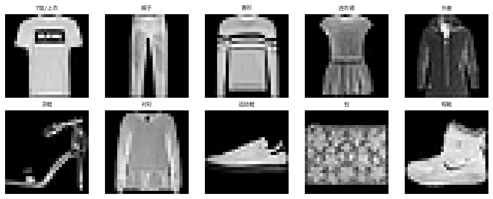
类别编号 0–9 分别表示 T恤/上衣、裤子、套衫、连衣裙、外套、凉鞋、衬衫、运动鞋、包和短靴。数据总体均衡,因此准确率有直观意义,但相似上衣类别之间仍可能出现系统性混淆。
图像可视化用于检查标签和方向,不应从少数图片推断模型已经学会某种固定语义。
CLASS_NAMES = ['T恤/上衣', '裤子', '套衫', '连衣裙', '外套', '凉鞋', '衬衫', '运动鞋', '包', '短靴']
counts = pd.Series(train_labels_all).value_counts().sort_index()
display(pd.DataFrame({'类别': CLASS_NAMES, '样本数': counts.to_numpy()}))
fig, axes = plt.subplots(2, 5, figsize=(10, 4))
for class_id, axis in enumerate(axes.ravel()):
    index = int(np.flatnonzero(train_labels_all == class_id)[0])
    axis.imshow(train_images_all[index], cmap='gray')
    axis.set_title(CLASS_NAMES[class_id], fontsize=8)
    axis.axis('off')
plt.tight_layout()
plt.show()
print('像素范围:', int(train_images_all.min()), int(train_images_all.max()))
| 类别 | 样本数 | |
|---|---|---|
| 0 | T恤/上衣 | 6000 |
| 1 | 裤子 | 6000 |
| 2 | 套衫 | 6000 |
| 3 | 连衣裙 | 6000 |
| 4 | 外套 | 6000 |
| 5 | 凉鞋 | 6000 |
| 6 | 衬衫 | 6000 |
| 7 | 运动鞋 | 6000 |
| 8 | 包 | 6000 |
| 9 | 短靴 | 6000 |
像素范围: 0 255
第 3 步:划分训练集、验证集与快速模式子集#
官方测试集不参与模型选择;程序从官方训练集中划分出验证集。快速模式从训练部分按类别比例选择子集,使每个类别保留相同数量的样本,从而缩短运行时间且不改变类别构成。图像转换为 \(n\times1\times28\times28\) 的四维数组,随后在模型内部展平为 \(n\times784\) 的矩阵。标签保持为一维整数向量,符合 CrossEntropyLoss 的输入要求。
这里不使用测试集计算任何预处理统计量,只把所有像素除以固定常数 255,因此测试集信息不会进入训练过程。
from sklearn.model_selection import train_test_split

all_index = np.arange(len(train_labels_all))
train_index, validation_index = train_test_split(all_index, test_size=10000, stratify=train_labels_all, random_state=SEED)
if FAST_MODE:
    train_index, _ = train_test_split(train_index, train_size=12000, stratify=train_labels_all[train_index], random_state=SEED)
    validation_index, _ = train_test_split(validation_index, train_size=3000, stratify=train_labels_all[validation_index], random_state=SEED)
    test_index, _ = train_test_split(np.arange(len(test_labels)), train_size=3000, stratify=test_labels, random_state=SEED)
else:
    test_index = np.arange(len(test_labels))

def make_tensor_set(images, labels, indices):
    X = torch.from_numpy(images[indices].copy()).float().unsqueeze(1) / 255.0
    y = torch.from_numpy(labels[indices].copy()).long()
    assert X.ndim == 4 and X.shape[1:] == (1, 28, 28)
    assert y.shape == (X.shape[0],)
    return TensorDataset(X, y)

train_set = make_tensor_set(train_images_all, train_labels_all, train_index)
validation_set = make_tensor_set(train_images_all, train_labels_all, validation_index)
test_set = make_tensor_set(test_images, test_labels, test_index)
print({'训练样本数': len(train_set), '验证样本数': len(validation_set), '测试样本数': len(test_set), '训练输入维度': tuple(train_set.tensors[0].shape)})
{'训练样本数': 12000, '验证样本数': 3000, '测试样本数': 3000, '训练输入维度': (12000, 1, 28, 28)}
第 4 步:最近类别均值基线#
先构造无需迭代优化的基线:对训练集中每个类别求平均图像,预测时选择欧氏距离最近的类别均值。它保留像素位置,但每类只有一个模板,无法表达同一服饰的多种形态。若神经网络不能明显超过它,应先检查数据、标签、损失和更新流程,而不是继续增加层数。
from sklearn.metrics import accuracy_score

X_train_flat = train_set.tensors[0].numpy().reshape(len(train_set), -1)
y_train_numpy = train_set.tensors[1].numpy()
X_validation_flat = validation_set.tensors[0].numpy().reshape(len(validation_set), -1)
y_validation_numpy = validation_set.tensors[1].numpy()
centroids = np.stack([X_train_flat[y_train_numpy == class_id].mean(axis=0) for class_id in range(10)])
distance = ((X_validation_flat[:, None, :] - centroids[None, :, :]) ** 2).sum(axis=2)
baseline_prediction = distance.argmin(axis=1)
print('最近类别均值验证准确率:', accuracy_score(y_validation_numpy, baseline_prediction))
assert centroids.shape == (10, 784)
最近类别均值验证准确率: 0.6846666666666666
第 5 步:稳定计算 Softmax 与多分类交叉熵#
对于一批输出层的线性运算结果 \(\boldsymbol{Z}\in\mathbb{R}^{n\times K}\),Softmax 在每个样本的类别方向上进行归一化:
从同一样本的所有线性运算结果中减去最大值不会改变 Softmax 概率,因为 Softmax 对所有分量共同增加或减少同一个常数保持不变;这样做还能避免直接计算很大的指数。真实类别对应概率的平均负对数就是多分类交叉熵。PyTorch 的 CrossEntropyLoss 在内部以数值稳定的方式组合 LogSoftmax 与负对数似然,因此模型最后应直接输出线性运算结果,不能预先再计算一次 Softmax。
def stable_softmax(logits):
    shifted = logits - logits.max(axis=1, keepdims=True)
    exponent = np.exp(shifted)
    return exponent / exponent.sum(axis=1, keepdims=True)

def multiclass_cross_entropy(logits, target):
    probability = stable_softmax(logits)
    return float(-np.log(np.clip(probability[np.arange(len(target)), target], 1e-12, 1)).mean())

probe_logits = np.array([[1000.0, 1001.0, 999.0], [-1000.0, -999.0, -1002.0]])
probe_probability = stable_softmax(probe_logits)
assert probe_probability.shape == probe_logits.shape
assert np.allclose(probe_probability.sum(axis=1), 1)
print('Softmax 概率:')
display(pd.DataFrame(probe_probability, columns=['类别 0', '类别 1', '类别 2']))
print('多分类交叉熵:', multiclass_cross_entropy(probe_logits, np.array([1, 0])))
Softmax 概率:
| 类别 0 | 类别 1 | 类别 2 | |
|---|---|---|---|
| 0 | 0.244728 | 0.665241 | 0.090031 |
| 1 | 0.259496 | 0.705385 | 0.035119 |
多分类交叉熵: 0.8783090906062834
第 6 步:定义全连接网络并核对维度#
模型依次进行 \(784\rightarrow128\rightarrow64\rightarrow10\) 的映射。Flatten 只把每幅二维图像的像素排成一个向量,不包含需要训练的参数;两个隐藏层使用 ReLU 引入非线性;输出层的 10 个线性运算结果分别对应 10 个类别。全连接层没有明确利用相邻像素之间的关系,这也是后续卷积神经网络案例的重要比较起点。
每次正式训练前,先用一个批次核对输入、展平结果、输出层线性运算结果和标签的维度。
class FashionMLP(nn.Module):
    def __init__(self):
        super().__init__()
        self.network = nn.Sequential(
            nn.Flatten(),
            nn.Linear(28 * 28, 128),
            nn.ReLU(),
            nn.Linear(128, 64),
            nn.ReLU(),
            nn.Linear(64, 10),
        )

    def forward(self, images):
        return self.network(images)

model = FashionMLP().to(DEVICE)
probe_images, probe_labels = next(iter(DataLoader(train_set, batch_size=32, shuffle=False)))
with torch.no_grad():
    probe_logits = model(probe_images.to(DEVICE))
assert probe_images.shape == (32, 1, 28, 28)
assert probe_logits.shape == (32, 10)
assert probe_labels.shape == (32,)
parameter_count = sum(parameter.numel() for parameter in model.parameters())
print({'输入维度': tuple(probe_images.shape), '线性运算结果维度': tuple(probe_logits.shape), '参数量': parameter_count})
{'输入维度': (32, 1, 28, 28), '线性运算结果维度': (32, 10), '参数量': 109386}
第 7 步:训练模式、评估模式与保存模型参数#
训练阶段调用 model.train(),计算梯度并更新参数;评估阶段调用 model.eval(),同时关闭梯度记录。当前网络没有 Dropout 或批量归一化(Batch Normalization,BatchNorm),但保留这套模式切换可以避免以后加入这些模块时得到错误结果。
每一轮都根据验证集交叉熵决定是否保存当前模型参数,不使用测试集选择训练轮数。快速模式训练 4 轮,完整模式训练 10 轮。若只是检查代码是否能够运行,可以进一步减少训练样本,但解释结果时必须说明所用的数据规模和训练轮数。
train_generator = torch.Generator().manual_seed(SEED)
train_loader = DataLoader(train_set, batch_size=128, shuffle=True, generator=train_generator)
validation_loader = DataLoader(validation_set, batch_size=256, shuffle=False)
test_loader = DataLoader(test_set, batch_size=256, shuffle=False)
criterion = nn.CrossEntropyLoss()
optimizer = torch.optim.Adam(model.parameters(), lr=1e-3)

def run_epoch(loader, training):
    model.train(training)
    total_loss = 0.0
    correct = 0
    total = 0
    context = torch.enable_grad() if training else torch.no_grad()
    with context:
        for images, labels in loader:
            images, labels = images.to(DEVICE), labels.to(DEVICE)
            logits = model(images)
            assert logits.shape == (labels.shape[0], 10)
            loss = criterion(logits, labels)
            if training:
                optimizer.zero_grad(set_to_none=True)
                loss.backward()
                optimizer.step()
            total_loss += loss.item() * labels.shape[0]
            correct += (logits.argmax(dim=1) == labels).sum().item()
            total += labels.shape[0]
    return total_loss / total, correct / total

history = []
best_state = None
best_validation_loss = np.inf
for epoch in range(1, (4 if FAST_MODE else 10) + 1):
    train_loss, train_accuracy = run_epoch(train_loader, True)
    validation_loss, validation_accuracy = run_epoch(validation_loader, False)
    history.append({'epoch': epoch, 'train_loss': train_loss, 'validation_loss': validation_loss, 'train_accuracy': train_accuracy, 'validation_accuracy': validation_accuracy})
    if validation_loss < best_validation_loss:
        best_validation_loss = validation_loss
        best_state = {key: value.detach().cpu().clone() for key, value in model.state_dict().items()}
model.load_state_dict(best_state)
history = pd.DataFrame(history)
history_display = history.rename(columns={'epoch': '训练轮次', 'train_loss': '训练损失', 'validation_loss': '验证损失', 'train_accuracy': '训练准确率', 'validation_accuracy': '验证准确率'})
display(history_display)
| 训练轮次 | 训练损失 | 验证损失 | 训练准确率 | 验证准确率 | |
|---|---|---|---|---|---|
| 0 | 1 | 1.035502 | 0.673659 | 0.642833 | 0.766333 |
| 1 | 2 | 0.601172 | 0.542547 | 0.791167 | 0.816667 |
| 2 | 3 | 0.514051 | 0.478985 | 0.821750 | 0.837333 |
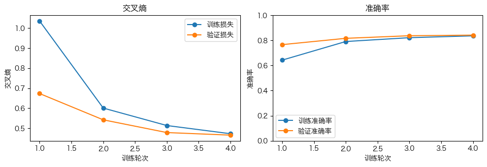
| 3 | 4 | 0.473151 | 0.466187 | 0.836500 | 0.842000 |
第 8 步:解释训练曲线#
训练与验证损失都下降,说明优化方向基本正确;训练继续下降而验证上升,则提示开始过拟合。准确率与交叉熵也可能给出不同信号:预测类别不变时,模型把错误概率变得更自信会恶化交叉熵,却不一定立刻改变准确率。因此检查点采用验证交叉熵,而不是只看训练准确率。
fig, axes = plt.subplots(1, 2, figsize=(10, 3.5))
history_display.plot(x='训练轮次', y=['训练损失', '验证损失'], marker='o', ax=axes[0], title='交叉熵')
history_display.plot(x='训练轮次', y=['训练准确率', '验证准确率'], marker='o', ax=axes[1], title='准确率')
axes[0].set_xlabel('训练轮次')
axes[0].set_ylabel('交叉熵')
axes[1].set_xlabel('训练轮次')
axes[1].set_ylabel('准确率')
axes[1].set_ylim(0, 1)
plt.tight_layout()
plt.show()
assert np.isfinite(history.select_dtypes('number').to_numpy()).all()
第 9 步:在模型确定后评价测试集并绘制混淆矩阵#
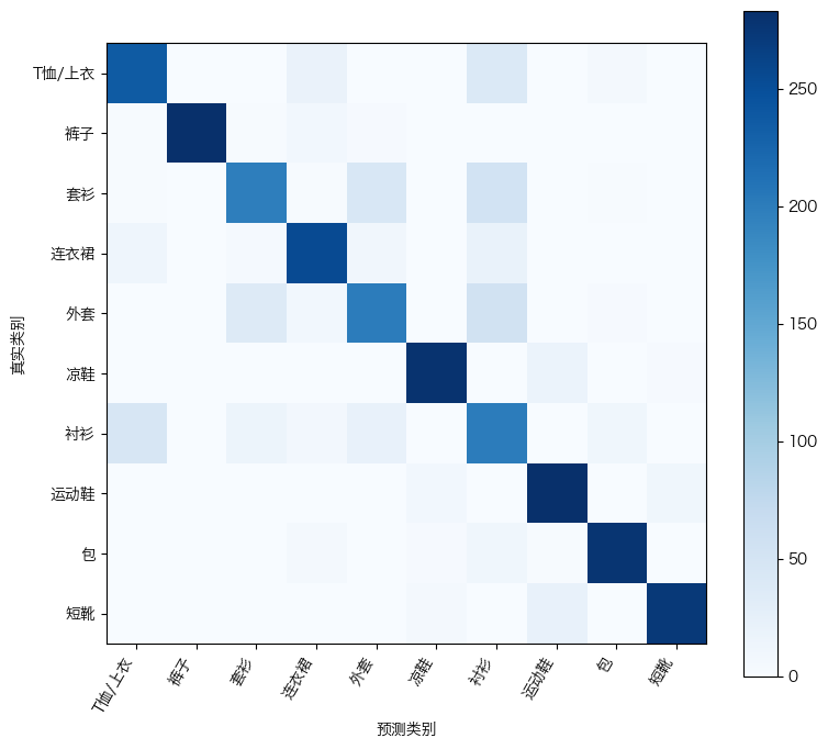
根据验证集确定要使用的模型参数后,只在测试集上评价一次。先收集输出层的线性运算结果,再计算 Softmax 概率;每个样本的 10 个类别概率之和应为 1。混淆矩阵的行表示真实类别,列表示预测类别,对角线表示分类正确的样本。相似服饰类别之间的非对角元素能够说明具体混淆方向,比单独一个准确率包含更多信息。
from sklearn.metrics import classification_report, confusion_matrix, log_loss

model.eval()
all_logits, all_targets = [], []
with torch.no_grad():
    for images, labels in test_loader:
        all_logits.append(model(images.to(DEVICE)).cpu())
        all_targets.append(labels)
test_logits = torch.cat(all_logits).numpy()
test_target = torch.cat(all_targets).numpy()
test_probability = stable_softmax(test_logits)
test_prediction = test_probability.argmax(axis=1)
assert test_probability.shape == (len(test_set), 10)
assert np.allclose(test_probability.sum(axis=1), 1, atol=1e-6)
print({'测试准确率': accuracy_score(test_target, test_prediction), '测试对数损失': log_loss(test_target, test_probability)})
report = pd.DataFrame(classification_report(test_target, test_prediction, target_names=CLASS_NAMES, output_dict=True)).T
report_display = report.rename(index={'accuracy': '准确率', 'macro avg': '宏平均', 'weighted avg': '加权平均'}, columns={'precision': '精确率', 'recall': '召回率', 'f1-score': 'F1 分数', 'support': '样本数'})
display(report_display)
confusion = confusion_matrix(test_target, test_prediction)
plt.figure(figsize=(8, 7))
plt.imshow(confusion, cmap='Blues')
plt.xticks(range(10), CLASS_NAMES, rotation=60, ha='right')
plt.yticks(range(10), CLASS_NAMES)
plt.xlabel('预测类别')
plt.ylabel('真实类别')
plt.colorbar()
plt.tight_layout()
plt.show()
{'测试准确率': 0.8263333333333334, '测试对数损失': 0.48312345147132874}
| 精确率 | 召回率 | F1 分数 | 样本数 | |
|---|---|---|---|---|
| T恤/上衣 | 0.786667 | 0.786667 | 0.786667 | 300.000000 |
| 裤子 | 0.992982 | 0.943333 | 0.967521 | 300.000000 |
| 套衫 | 0.772549 | 0.656667 | 0.709910 | 300.000000 |
| 连衣裙 | 0.841060 | 0.846667 | 0.843854 | 300.000000 |
| 外套 | 0.713262 | 0.663333 | 0.687392 | 300.000000 |
| 凉鞋 | 0.942568 | 0.930000 | 0.936242 | 300.000000 |
| 衬衫 | 0.531915 | 0.666667 | 0.591716 | 300.000000 |
| 运动鞋 | 0.873065 | 0.940000 | 0.905297 | 300.000000 |
| 包 | 0.926421 | 0.923333 | 0.924875 | 300.000000 |
| 短靴 | 0.954386 | 0.906667 | 0.929915 | 300.000000 |
| 准确率 | 0.826333 | 0.826333 | 0.826333 | 0.826333 |
| 宏平均 | 0.833487 | 0.826333 | 0.828339 | 3000.000000 |
| 加权平均 | 0.833487 | 0.826333 | 0.828339 | 3000.000000 |
第 10 步:分析预测概率较高的错误样本#
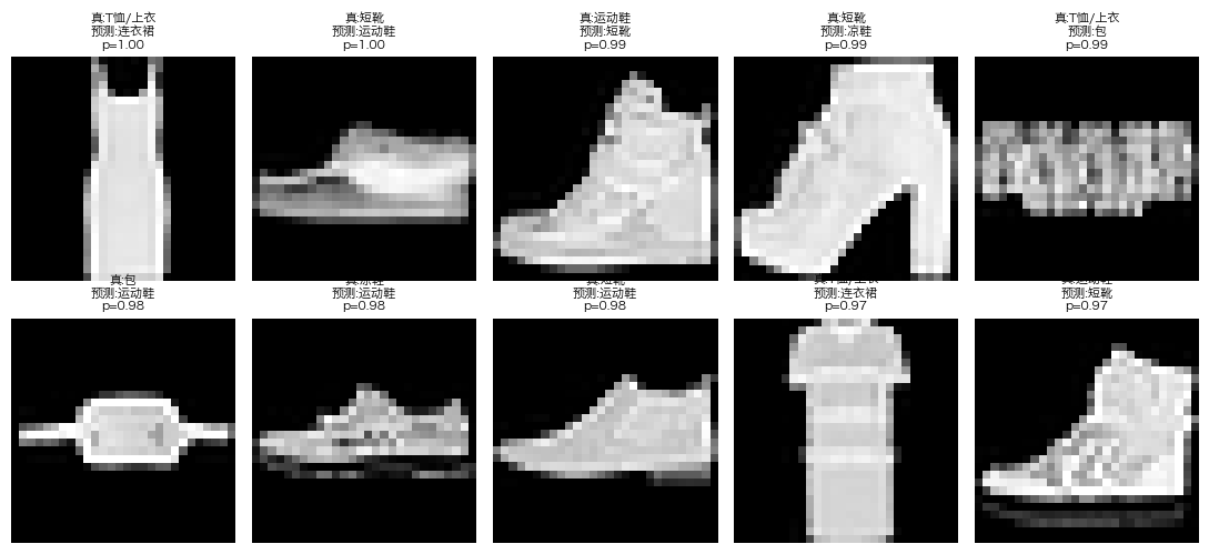
下面选出模型给出的最大类别概率较高、但预测仍然错误的图像。较高概率只说明模型把较多概率集中在某一个类别上,并不能证明预测一定可靠。若错误集中在衬衫、T恤/上衣、套衫和外套之间,说明展平后的全连接网络可能难以充分利用局部纹理和轮廓;这与卷积神经网络利用局部连接的思想直接相关。
这些测试错误只能用于描述模型的局限,不能再用来选择超参数,否则测试集实际上就参与了模型选择。
wrong = np.flatnonzero(test_prediction != test_target)
wrong = wrong[np.argsort(test_probability[wrong].max(axis=1))[::-1]]
fig, axes = plt.subplots(2, 5, figsize=(11, 5))
selected = wrong[:10]
for axis, local_index in zip(axes.ravel(), selected):
    original_index = test_index[local_index]
    axis.imshow(test_images[original_index], cmap='gray')
    axis.set_title(f'真:{CLASS_NAMES[test_target[local_index]]}\n预测:{CLASS_NAMES[test_prediction[local_index]]}\np={test_probability[local_index].max():.2f}', fontsize=8)
    axis.axis('off')
for axis in axes.ravel()[len(selected):]:
    axis.axis('off')
plt.tight_layout()
plt.show()
print('测试错误数:', len(wrong))
测试错误数: 521
结论、局限与常见错误#
稳定计算 Softmax 时,应从每个样本的全部线性运算结果中减去该样本的最大值;不能把不同样本混在一起进行类别归一化。
CrossEntropyLoss的输入是输出层的线性运算结果和一维整数标签;提前计算 Softmax,或者把类别编号错误地转换为浮点数,都是常见错误。展平后的全连接网络不再明确利用像素在二维图像中的相邻位置关系,不能据此认为它是图像任务的最佳结构。
快速模式的子集结果只用于教学演示,不能与使用完整数据和更长训练时间得到的论文结果直接比较。
Fashion-MNIST 图像较小、只有灰度且背景简单,不能代表真实服饰识别中的光照、姿态、遮挡和人群差异。
单次数据划分和单个随机种子的结果不足以说明模型差异具有普遍性;正式比较应使用多个随机种子重复运行,并报告计算时间和内存等成本。
综合练习#
手算三个类别的线性运算结果 \((2,1,-1)\) 对应的稳定 Softmax 概率,以及真实类别为第 2 类时的交叉熵。
用中心差分检查 Softmax 交叉熵对输出层线性运算结果的梯度 \((\boldsymbol{P}-\boldsymbol{Y})/n\)。
比较没有隐藏层的 Softmax 回归、当前 MLP 和参数量接近的小型卷积神经网络;三个模型使用相同的数据划分、随机种子和参数更新次数。
在隐藏层中加入 Dropout,验证调用
train()时同一个输入可能得到不同输出,而调用eval()时输出保持稳定。找出召回率最低的三个类别,并根据混淆矩阵说明它们主要被预测成哪些类别;不要根据测试集结果返回去调整模型。
使用完整模式训练,记录训练时间、最大内存占用、参数量和测试指标,并说明这些结果为什么不能与快速模式的短训练结果直接比较。