案例 15:OGBN-Arxiv 节点分类——从多层感知机到消息传递#
学习目标与记号#
节点分类的输入不仅包括节点特征,还包括节点之间的引用关系。本案例用论文引用网络讨论结构信息何时能帮助主题分类。本案例的学习目标包括:
核对特征矩阵 \(\boldsymbol{X}\in\mathbb{R}^{n\times d}\)、边索引和标签的维度;
解释“消息—聚合—更新”,用纯 PyTorch 实现图卷积网络(GCN)、图采样聚合网络(GraphSAGE)与单头图注意力网络(GAT);
用无结构 MLP 作公平基线,只在验证集选择模型,最后一次性评价测试集;
验证置换等变性,并用层数增加后的相似度观察过度平滑;
说明 OGBN-Arxiv 官方时间划分为何比随机划分更接近“用过去预测未来”。
本案例只用于算法教学,不用于评价论文、作者或研究质量。
数据来源、许可与运行模式#
数据集:OGBN-Arxiv
匿名直接下载:https://snap.stanford.edu/ogb/data/nodeproppred/arxiv.zip
许可:ODC-BY;使用时还应引用 OGB 与原始 MAG/Arxiv 来源。
快速模式是默认教学模式:仍下载官方压缩包,但只从官方训练集、验证集和测试集中分别选择一部分节点,再构造由这些节点及其内部边组成的诱导子图;只使用中央处理器(central processing unit,CPU)也可验证核心公式。完整模式使用全部节点,建议至少准备 8 GB 内存并使用图形处理器(graphics processing unit,GPU)。缓存写入 AI_COURSE_DATA_DIR;若未设置,则写入用户缓存,不写入课程源码目录。
诱导子图会删除通向未抽样节点的边,因此其结果不能冒充 OGB 官方排行榜结果。
from pathlib import Path
import copy
import gzip
import hashlib
import os
import random
import urllib.request
import zipfile

import matplotlib.pyplot as plt
import numpy as np
import pandas as pd
import torch
from sklearn.metrics import accuracy_score, f1_score

SEED = 42
FAST_MODE = os.getenv("AI_COURSE_FAST_MODE", os.getenv("FAST_MODE", "1")) != "0"
random.seed(SEED)
np.random.seed(SEED)
torch.manual_seed(SEED)

cache_root = Path(
    os.environ.get(
        "AI_COURSE_DATA_DIR",
        Path(os.environ.get("XDG_CACHE_HOME", Path.home() / ".cache")) / "ai-course-cases",
    )
).expanduser()
cache_root.mkdir(parents=True, exist_ok=True)
device = torch.device("cuda" if (not FAST_MODE and torch.cuda.is_available()) else "cpu")
print({"快速模式": FAST_MODE, "计算设备": str(device), "缓存目录": str(cache_root)})
{'快速模式': True, '计算设备': 'cpu', '缓存目录': '/Users/zw/.cache/ai-course-cases'}
第 1 步:下载并读取 OGB 原始文件#
下面只读取 ZIP 中需要的 gzip CSV,不把整个压缩包解压到源码树。下载采用临时文件后原子替换,避免中断后留下“看似完整”的坏文件;同时打印 SHA-256,便于记录本次快照。
OGB 图属性约定为:
node-feat.csv.gz:\((n,d)\) 节点特征;
edge.csv.gz:\((m,2)\) 有向边,每行依次是发送端(source)与接收端(target);
node-label.csv.gz:\((n,1)\) 类别;
split/time 下的文件:官方时间划分节点编号。
测试标签只在模型和超参数冻结后进入最终评价。
DATA_URL = "https://snap.stanford.edu/ogb/data/nodeproppred/arxiv.zip"
archive = cache_root / "ogbn_arxiv.zip"

def download_cached(url, target):
    if not target.exists():
        temporary = target.with_suffix(target.suffix + ".part")
        request = urllib.request.Request(url, headers={"User-Agent": "ai-course-case/1.0"})
        with urllib.request.urlopen(request, timeout=120) as response, temporary.open("wb") as out:
            while chunk := response.read(1024 * 1024):
                out.write(chunk)
        temporary.replace(target)
    digest = hashlib.sha256(target.read_bytes()).hexdigest()
    size_mib = round(target.stat().st_size / 2**20, 1)
    print(f"文件:{target.name};大小:{size_mib} 兆字节;SHA-256:{digest}")
    return target

def find_member(names, suffix):
    matches = [name for name in names if name.endswith(suffix)]
    if len(matches) != 1:
        raise FileNotFoundError(f"需要唯一的 {suffix},实际找到 {matches[:5]}")
    return matches[0]

def read_gzip_csv(zf, suffix, dtype):
    member = find_member(zf.namelist(), suffix)
    with zf.open(member) as raw, gzip.GzipFile(fileobj=raw) as uncompressed:
        return pd.read_csv(uncompressed, header=None).to_numpy(dtype=dtype)

download_cached(DATA_URL, archive)
with zipfile.ZipFile(archive) as zf:
    X_all = read_gzip_csv(zf, "/raw/node-feat.csv.gz", np.float32)
    edge_rows = read_gzip_csv(zf, "/raw/edge.csv.gz", np.int64)
    y_all = read_gzip_csv(zf, "/raw/node-label.csv.gz", np.int64).reshape(-1)
    split_global = {
        "train": read_gzip_csv(zf, "/split/time/train.csv.gz", np.int64).reshape(-1),
        "valid": read_gzip_csv(zf, "/split/time/valid.csv.gz", np.int64).reshape(-1),
        "test": read_gzip_csv(zf, "/split/time/test.csv.gz", np.int64).reshape(-1),
    }

if edge_rows.shape[1] != 2 and edge_rows.shape[0] == 2:
    edge_rows = edge_rows.T
if edge_rows.ndim != 2 or edge_rows.shape[1] != 2:
    raise ValueError(f"无法识别边的维度:{edge_rows.shape}")
print("完整数据的维度:", X_all.shape, edge_rows.shape, y_all.shape)
official_split_sizes = {"训练集": len(split_global["train"]),
                        "验证集": len(split_global["valid"]),
                        "测试集": len(split_global["test"])}
print("官方划分:", official_split_sizes)
文件:ogbn_arxiv.zip;大小:79.2 兆字节;SHA-256:49f85c801589ecdcc52cfaca99693aaea7b8af16a9ac3f41dd85a5f3193fe276
完整数据的维度: (169343, 128) (1166243, 2) (169343,)
官方划分: {'训练集': 90941, '验证集': 29799, '测试集': 48603}
第 2 步:检查图数据#
普通表格检查“行数 × 列数”;图数据还必须检查边端点范围、自环、方向和类别不平衡。引用边原本有方向,教学模型随后把它对称化,使一篇论文能聚合“引用与被引用”的局部上下文。这个决定改变模型假设,必须写明。
分别检查官方训练集、验证集和测试集中的类别分布,可以观察较晚发表的论文是否具有不同的主题比例。
assert len(X_all) == len(y_all)
assert edge_rows.min() >= 0 and edge_rows.max() < len(X_all)
audit = []
split_names = {"train": "训练集", "valid": "验证集", "test": "测试集"}
for part, indices in split_global.items():
    counts = np.bincount(y_all[indices], minlength=int(y_all.max()) + 1)
    audit.append({
        "数据集合": split_names[part],
        "节点数": len(indices),
        "出现的类别数": int((counts > 0).sum()),
        "最大类别占比": float(counts.max() / counts.sum()),
    })
display(pd.DataFrame(audit))
print("特征有限值比例:", np.isfinite(X_all).mean())
print("有向边数:", len(edge_rows), "原始自环数:", int((edge_rows[:, 0] == edge_rows[:, 1]).sum()))
| 数据集合 | 节点数 | 出现的类别数 | 最大类别占比 | |
|---|---|---|---|---|
| 0 | 训练集 | 90941 | 40 | 0.179061 |
| 1 | 验证集 | 29799 | 40 | 0.229739 |
| 2 | 测试集 | 48603 | 40 | 0.220974 |
特征有限值比例: 1.0
有向边数: 1166243 原始自环数: 0
第 3 步:保留官方时间划分,构造教学子图#
随机拆分会让同一时期、甚至紧密引用的论文同时进入训练和测试,容易高估面向未来的泛化。官方时间划分把较早论文用于训练、较晚论文用于验证和测试。
快速模式在每个官方集合内部固定随机抽样,再取诱导子图。标准化只使用训练节点的统计量:
节点编号映射和选边只是结构整理,不读取测试标签。
rng = np.random.default_rng(SEED)
caps = {"train": 4000, "valid": 1000, "test": 1000}

if FAST_MODE:
    selected = {
        name: np.sort(rng.choice(idx, size=min(caps[name], len(idx)), replace=False))
        for name, idx in split_global.items()
    }
    keep_global = np.unique(np.concatenate(list(selected.values())))
else:
    selected = {name: idx.copy() for name, idx in split_global.items()}
    keep_global = np.arange(len(X_all), dtype=np.int64)

global_to_local = np.full(len(X_all), -1, dtype=np.int64)
global_to_local[keep_global] = np.arange(len(keep_global))
mapped_edges = global_to_local[edge_rows]
inside = (mapped_edges[:, 0] >= 0) & (mapped_edges[:, 1] >= 0)
edge_local = mapped_edges[inside].T
split_local = {
    name: torch.as_tensor(global_to_local[idx], dtype=torch.long, device=device)
    for name, idx in selected.items()
}

X_small = X_all[keep_global].copy()
y_small = y_all[keep_global].copy()
train_np = split_local["train"].cpu().numpy()
mu = X_small[train_np].mean(axis=0, keepdims=True)
sd = X_small[train_np].std(axis=0, keepdims=True)
X_small = (X_small - mu) / np.where(sd > 1e-8, sd, 1.0)

X = torch.as_tensor(X_small, dtype=torch.float32, device=device)
y = torch.as_tensor(y_small, dtype=torch.long, device=device)
edge_index = torch.as_tensor(edge_local, dtype=torch.long, device=device)
print("教学图:", {"节点数": len(X), "特征数": X.shape[1], "诱导边数": edge_index.shape[1]})
print("局部划分:", {split_names[k]: len(v) for k, v in split_local.items()})
教学图: {'节点数': 6000, '特征数': 128, '诱导边数': 1755}
局部划分: {'训练集': 4000, '验证集': 1000, '测试集': 1000}
第 4 步:无结构 MLP 基线#
多层感知机(MLP)对每个节点独立计算 \(f(\boldsymbol x_i)\),完全看不到边。它回答关键对照问题:提升来自图结构,还是节点文本特征本身已经足够?
所有模型使用相同的标准化特征、官方划分、隐藏层宽度和验证集提前停止规则。输出层先得到未归一化的线性运算结果,交叉熵函数在内部使用数值稳定的 log-softmax 计算。
class MLP(torch.nn.Module):
    def __init__(self, in_dim, hidden_dim, out_dim, dropout=0.35):
        super().__init__()
        self.net = torch.nn.Sequential(
            torch.nn.Linear(in_dim, hidden_dim),
            torch.nn.ReLU(),
            torch.nn.Dropout(dropout),
            torch.nn.Linear(hidden_dim, out_dim),
        )

    def forward(self, x, adjacency=None, edges=None):
        return self.net(x)

num_classes = int(y.max().item()) + 1
demo_logits = MLP(X.shape[1], 32, num_classes)(X[:7])
assert demo_logits.shape == (7, num_classes)
print("多层感知机维度核验:", tuple(X[:7].shape), "→", tuple(demo_logits.shape))
多层感知机维度核验: (7, 128) → (7, 40)
第 5 步:自环、归一化与置换等变性#
GCN 使用加自环后的 \(\widetilde A=A+I\) 和对称归一化:
代码以稀疏 COO 保存“行是接收节点、列是发送节点”,不会创建 \(n\times n\) 稠密矩阵。GraphSAGE 则先求邻居均值,再把自身与邻居表示拼接。
若同时置换节点行和邻接矩阵行列,消息传递结果会以相同方式置换,即 \(P(AX)=(PAP^\mathsf T)(PX)\)。这叫置换等变,不是输出完全不变。
def make_graph_operators(edge_index, n):
    src, dst = edge_index
    nodes = torch.arange(n, device=device)
    src_sym = torch.cat([src, dst, nodes])
    dst_sym = torch.cat([dst, src, nodes])
    indices = torch.stack([dst_sym, src_sym])

    degree = torch.bincount(dst_sym, minlength=n).float().clamp_min(1)
    gcn_weight = degree[dst_sym].rsqrt() * degree[src_sym].rsqrt()
    mean_weight = 1.0 / degree[dst_sym]
    A_gcn = torch.sparse_coo_tensor(indices, gcn_weight, (n, n)).coalesce()
    A_mean = torch.sparse_coo_tensor(indices, mean_weight, (n, n)).coalesce()
    return A_gcn, A_mean, torch.stack([src_sym, dst_sym])

A_gcn, A_mean, message_edges = make_graph_operators(edge_index, len(X))

tiny_A = torch.tensor([[1., 1., 0.], [1., 1., 1.], [0., 1., 1.]])
tiny_X = torch.arange(6, dtype=torch.float32).reshape(3, 2)
perm = torch.tensor([2, 0, 1])
P = torch.eye(3)[perm]
assert torch.allclose(P @ (tiny_A @ tiny_X), (P @ tiny_A @ P.T) @ (P @ tiny_X))
print("置换等变检查通过;稀疏邻接非零元:", A_gcn._nnz())
置换等变检查通过;稀疏邻接非零元: 9462
第 6 步:三种图消息传递方法#
GCN 用固定的度归一化权重;GraphSAGE 把自身和邻居均值拼接;GAT 对边 \(j\to i\) 学习注意力:
下面使用稀疏乘法以及 PyTorch 的 index-add 和 scatter-reduce 接口实现。这适合教学子图,但不替代 PyG 等高度优化的全量工具。
class GCNNet(torch.nn.Module):
    def __init__(self, in_dim, hidden_dim, out_dim, dropout=0.35):
        super().__init__()
        self.lin1 = torch.nn.Linear(in_dim, hidden_dim, bias=False)
        self.lin2 = torch.nn.Linear(hidden_dim, out_dim, bias=False)
        self.dropout = dropout

    def forward(self, x, adjacency, edges=None):
        h = torch.relu(self.lin1(torch.sparse.mm(adjacency, x)))
        h = torch.dropout(h, self.dropout, self.training)
        return self.lin2(torch.sparse.mm(adjacency, h))

class SAGENet(torch.nn.Module):
    def __init__(self, in_dim, hidden_dim, out_dim, dropout=0.35):
        super().__init__()
        self.lin1 = torch.nn.Linear(2 * in_dim, hidden_dim)
        self.lin2 = torch.nn.Linear(2 * hidden_dim, out_dim)
        self.dropout = dropout

    def forward(self, x, adjacency, edges=None):
        neighbor = torch.sparse.mm(adjacency, x)
        h = torch.relu(self.lin1(torch.cat([x, neighbor], dim=1)))
        h = torch.dropout(h, self.dropout, self.training)
        neighbor_h = torch.sparse.mm(adjacency, h)
        return self.lin2(torch.cat([h, neighbor_h], dim=1))

class GATLayer(torch.nn.Module):
    def __init__(self, in_dim, out_dim):
        super().__init__()
        self.linear = torch.nn.Linear(in_dim, out_dim, bias=False)
        self.a_src = torch.nn.Parameter(torch.empty(out_dim))
        self.a_dst = torch.nn.Parameter(torch.empty(out_dim))
        torch.nn.init.xavier_uniform_(self.linear.weight)
        torch.nn.init.normal_(self.a_src, std=0.1)
        torch.nn.init.normal_(self.a_dst, std=0.1)

    def forward(self, x, edges):
        src, dst = edges
        z = self.linear(x)
        score = torch.nn.functional.leaky_relu(
            (z[src] * self.a_src).sum(1) + (z[dst] * self.a_dst).sum(1), 0.2
        )
        maximum = torch.full((len(x),), -torch.inf, device=x.device)
        maximum.scatter_reduce_(0, dst, score, reduce="amax", include_self=True)
        exp_score = torch.exp(score - maximum[dst])
        denominator = torch.zeros(len(x), device=x.device)
        denominator.index_add_(0, dst, exp_score)
        alpha = exp_score / denominator[dst].clamp_min(1e-12)
        out = torch.zeros_like(z)
        out.index_add_(0, dst, alpha[:, None] * z[src])
        return out

class GATNet(torch.nn.Module):
    def __init__(self, in_dim, hidden_dim, out_dim, dropout=0.35):
        super().__init__()
        self.gat1 = GATLayer(in_dim, hidden_dim)
        self.gat2 = GATLayer(hidden_dim, out_dim)
        self.dropout = dropout

    def forward(self, x, adjacency=None, edges=None):
        h = torch.relu(self.gat1(x, edges))
        h = torch.dropout(h, self.dropout, self.training)
        return self.gat2(h, edges)
第 7 步:统一训练协议#
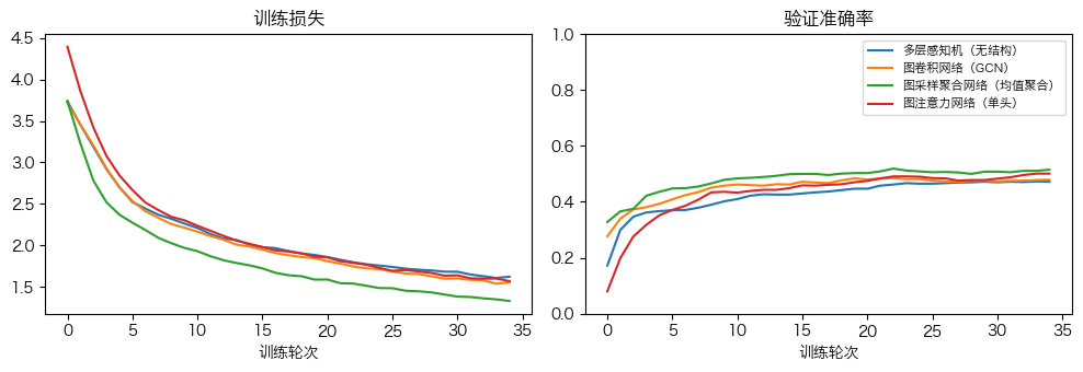
每次只在训练节点计算损失;验证准确率用于早停并保存最佳状态。测试节点可以参与整图消息传递,这是 OGB 的传导式设置,但测试标签绝不进入梯度或模型选择。若部署对象是完全不可见的新节点,应改成归纳式子图评估。
四个模型共享种子、隐藏宽度、轮数和评价函数。快速模式轮数较少,重点是可运行的概念实验,不是刷新排行榜。
def evaluate_indices(logits, indices):
    return float((logits[indices].argmax(1) == y[indices]).float().mean().item())

def fit_model(model, epochs, learning_rate=0.01, weight_decay=5e-4):
    model = model.to(device)
    optimizer = torch.optim.Adam(model.parameters(), lr=learning_rate, weight_decay=weight_decay)
    best_state, best_valid, stale = None, -1.0, 0
    history = []
    for epoch in range(epochs):
        model.train()
        optimizer.zero_grad()
        adjacency = A_mean if isinstance(model, SAGENet) else (None if isinstance(model, MLP) else A_gcn)
        logits = model(X, adjacency, message_edges)
        loss = torch.nn.functional.cross_entropy(logits[split_local["train"]], y[split_local["train"]])
        loss.backward()
        optimizer.step()

        model.eval()
        with torch.no_grad():
            logits = model(X, adjacency, message_edges)
            train_acc = evaluate_indices(logits, split_local["train"])
            valid_acc = evaluate_indices(logits, split_local["valid"])
        history.append((epoch, float(loss.item()), train_acc, valid_acc))
        if valid_acc > best_valid + 1e-5:
            best_valid = valid_acc
            best_state = copy.deepcopy(model.state_dict())
            stale = 0
        else:
            stale += 1
        if stale >= 12:
            break
    model.load_state_dict(best_state)
    return model, pd.DataFrame(history, columns=["训练轮次", "训练损失", "训练准确率", "验证准确率"])

epochs = 35 if FAST_MODE else 200
hidden = 48 if FAST_MODE else 128
model_factories = {
    "多层感知机(无结构)": lambda: MLP(X.shape[1], hidden, num_classes),
    "图卷积网络(GCN)": lambda: GCNNet(X.shape[1], hidden, num_classes),
    "图采样聚合网络(均值聚合)": lambda: SAGENet(X.shape[1], hidden, num_classes),
    "图注意力网络(单头)": lambda: GATNet(X.shape[1], hidden, num_classes),
}
trained, histories = {}, {}
for name, factory in model_factories.items():
    torch.manual_seed(SEED)
    trained[name], histories[name] = fit_model(factory(), epochs=epochs)
    print(name, "最佳验证准确率", histories[name]["验证准确率"].max())

fig, axes = plt.subplots(1, 2, figsize=(10, 3.5))
for name, hist in histories.items():
    axes[0].plot(hist["训练轮次"], hist["训练损失"], label=name)
    axes[1].plot(hist["训练轮次"], hist["验证准确率"], label=name)
axes[0].set(title="训练损失", xlabel="训练轮次")
axes[1].set(title="验证准确率", xlabel="训练轮次", ylim=(0, 1))
axes[1].legend(fontsize=8)
plt.tight_layout()
多层感知机(无结构) 最佳验证准确率 0.4729999899864197
图卷积网络(GCN) 最佳验证准确率 0.48500001430511475
图采样聚合网络(均值聚合) 最佳验证准确率 0.5189999938011169
图注意力网络(单头) 最佳验证准确率 0.5009999871253967
第 8 步:确定模型与训练方案后评价测试集#
准确率与 OGB 官方指标一致;宏平均 F1 分数给每个主题类别相同的权重,可以发现样本较多的类别是否掩盖了样本较少类别的表现。这里先根据验证集确定全部模型,再读取测试标签。
GNN 明显优于 MLP 时,局部引用结构提供了增量信息;两者接近也不等于“图无用”,还可能因为教学子图删边、训练预算小或节点特征很强。GAT 更灵活但也更难优化,并不保证最好。
rows = []
for name, model in trained.items():
    model.eval()
    with torch.no_grad():
        adjacency = A_mean if isinstance(model, SAGENet) else (None if isinstance(model, MLP) else A_gcn)
        logits = model(X, adjacency, message_edges)
    idx = split_local["test"]
    truth = y[idx].cpu().numpy()
    prediction = logits[idx].argmax(1).cpu().numpy()
    rows.append({
        "模型": name,
        "测试准确率": accuracy_score(truth, prediction),
        "测试宏平均F1分数": f1_score(truth, prediction, average="macro", zero_division=0),
        "参数量": sum(p.numel() for p in model.parameters()),
    })
results = pd.DataFrame(rows).sort_values("测试准确率", ascending=False)
display(results.style.format({"测试准确率": "{:.3f}", "测试宏平均F1分数": "{:.3f}"}))
| 模型 | 测试准确率 | 测试宏平均F1分数 | 参数量 | |
|---|---|---|---|---|
| 3 | 图注意力网络(单头) | 0.506 | 0.220 | 8240 |
| 1 | 图卷积网络(GCN) | 0.504 | 0.208 | 8064 |
| 2 | 图采样聚合网络(均值聚合) | 0.499 | 0.231 | 16216 |
| 0 | 多层感知机(无结构) | 0.470 | 0.205 | 8152 |
第 9 步:传播深度与过度平滑#
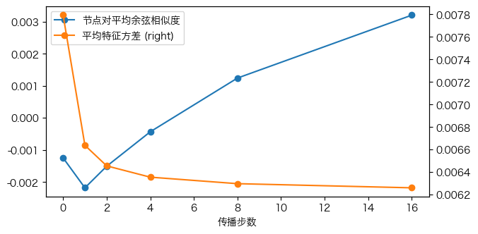
反复施加归一化邻接会不断混合邻居。层数过深时,连通区域内节点表示趋同,可区分性下降。我们记录随机节点对平均余弦相似度和跨节点特征方差。
这是“传播算子自身”的诊断,不等于深层 GNN 必然失败;残差、归一化、跳连和可学习权重都可能缓解问题。
def pair_cosine_mean(h, pairs=1000):
    local_rng = np.random.default_rng(SEED)
    a = torch.as_tensor(local_rng.integers(0, len(h), size=pairs), device=h.device)
    b = torch.as_tensor(local_rng.integers(0, len(h), size=pairs), device=h.device)
    return float(torch.nn.functional.cosine_similarity(h[a], h[b], dim=1).mean().item())

smooth_rows = []
h = torch.nn.functional.normalize(X, dim=1)
for layer in range(17):
    if layer in {0, 1, 2, 4, 8, 16}:
        smooth_rows.append({
            "传播步数": layer,
            "节点对平均余弦相似度": pair_cosine_mean(h),
            "平均特征方差": float(h.var(dim=0).mean().item()),
        })
    h = torch.sparse.mm(A_gcn, h)
smooth = pd.DataFrame(smooth_rows)
display(smooth)
smooth.plot(x="传播步数", y=["节点对平均余弦相似度", "平均特征方差"],
            secondary_y="平均特征方差", marker="o", figsize=(7, 3.5));
| 传播步数 | 节点对平均余弦相似度 | 平均特征方差 | |
|---|---|---|---|
| 0 | 0 | -0.001249 | 0.007793 |
| 1 | 1 | -0.002183 | 0.006637 |
| 2 | 2 | -0.001509 | 0.006455 |
| 3 | 4 | -0.000435 | 0.006355 |
| 4 | 8 | 0.001241 | 0.006297 |
| 5 | 16 | 0.003203 | 0.006260 |
结论、局限与常见错误#
本案例在其他条件相同的情况下,只改变模型是否使用边,借此比较图结构对分类结果的影响,但结论有以下边界:
快速模式是删边后的诱导子图,不能与 OGB 全量成绩比较;
GAT 只有单头,未使用邻居采样、批训练和成熟稀疏算子;
传导式评估允许测试节点特征和无标签结构参与传播,不能直接外推到完全新图;
简单邻居平均依赖局部同质性,异质图上可能有害;
若看过测试结果再改轮数或隐藏宽度,测试集就已变成验证集。
常见错误:写反边方向、忘记自环、创建稠密邻接导致内存爆炸、用全体节点拟合标准化统计量,以及把置换等变误称为置换不变。
综合练习#
保持其他设置不变,分别移除自环和对称归一化,解释验证曲线差异。
把 GAT 扩展为 4 个注意力头,核对每个头和拼接后张量的维度。
比较 1、2、4 层 GCN,同时报告验证准确率与节点余弦相似度。
构造严格归纳式实验:训练时移除验证、测试节点及相关边。
关闭快速模式后接入 OGB 官方评价程序;记录硬件、软件版本、随机种子和运行时间,不把完整数据结果与教学子图结果混在一起。