案例 18:真实二维数据上的分数模型、随机微分方程、条件引导与 DDIM#
学习目标与记号#
高维图像会让扩散轨迹难以直接观察。本案例先将 Palmer Penguins 数据集的两个连续测量标准化到二维平面,直接观察分数向量场和反向时间轨迹。随后用同一个噪声预测框架连接随机微分方程(stochastic differential equation,SDE)、类别条件、无分类器引导(classifier-free guidance,CFG)与去噪扩散隐式模型(denoising diffusion implicit model,DDIM)。本案例的学习目标包括:
解释分数 \(\nabla_{\boldsymbol{x}}\log p_t(\boldsymbol{x})\) 指向概率密度增加最快的方向,而不是分类模型对输入的梯度;
推导去噪分数匹配与噪声预测的比例关系;
区分方差爆炸(variance exploding,VE)与方差保持(variance preserving,VP)SDE,理解反向时间 SDE 与概率流常微分方程(ordinary differential equation,ODE)的随机路径和确定性路径;
实现类别条件噪声预测器与 CFG;
实现 DDPM 与 DDIM 更新,比较随机性、步数和条件强度;
说明 U-Net、潜空间扩散模型(latent diffusion model,LDM)与扩散 Transformer(Diffusion Transformer,DiT)改变了哪些网络或数据表示,以及哪些核心概率结构保持不变。
默认的快速模式可在中央处理器(central processing unit,CPU)上用几分钟完成二维教学实验。Fashion-MNIST 只在末尾用于检查“迁移到图像”时的数据接口与维度,不进行计算量很大的图像模型训练。
数据来源、许可与任务边界#
主数据是 Palmer Penguins:
匿名直链:https://raw.githubusercontent.com/allisonhorst/palmerpenguins/main/inst/extdata/penguins.csv
许可:CC0。
图像扩展使用 Fashion-MNIST 训练图像与标签:
https://storage.googleapis.com/tensorflow/tf-keras-datasets/train-images-idx3-ubyte.gz
https://storage.googleapis.com/tensorflow/tf-keras-datasets/train-labels-idx1-ubyte.gz
许可:MIT。
所有文件缓存在 AI_COURSE_DATA_DIR 指定的目录中,或用户缓存目录中。企鹅物种只作为条件标签,二维特征为喙长 bill_length_mm 与鳍长 flipper_length_mm;本案例不作生态因果推断,也不用于个体识别。
from pathlib import Path
import copy
import gzip
import hashlib
import os
import random
import struct
import urllib.request

import matplotlib.pyplot as plt
import numpy as np
import pandas as pd
import torch
from sklearn.model_selection import train_test_split
from sklearn.preprocessing import StandardScaler
from torch.utils.data import DataLoader, TensorDataset

SEED = 42
FAST_MODE = os.getenv("AI_COURSE_FAST_MODE", os.getenv("FAST_MODE", "1")) != "0"
random.seed(SEED)
np.random.seed(SEED)
torch.manual_seed(SEED)
device = torch.device("cuda" if (not FAST_MODE and torch.cuda.is_available()) else "cpu")

cache_root = Path(
    os.environ.get(
        "AI_COURSE_DATA_DIR",
        Path(os.environ.get("XDG_CACHE_HOME", Path.home() / ".cache")) / "ai-course-cases",
    )
).expanduser()
cache_root.mkdir(parents=True, exist_ok=True)
print({"快速模式": FAST_MODE, "计算设备": str(device), "缓存目录": str(cache_root)})
{'快速模式': True, '计算设备': 'cpu', '缓存目录': '/Users/zw/.cache/ai-course-cases'}
第 1 步:下载二维真实数据并记录快照#
下载函数先写入临时文件,成功后再替换正式文件,并打印 SHA-256 校验值。逗号分隔值(comma-separated values,CSV)文件使用公开链接,不需要登录、应用程序编程接口(application programming interface,API)密钥或本机绝对路径。
读入后只保留三个物种标签和两个连续特征,并显式删除这三列中的缺失行。删除规则在拆分之前定义,但标准化参数必须稍后只用训练集拟合。
PENGUINS_URL = "https://raw.githubusercontent.com/allisonhorst/palmerpenguins/main/inst/extdata/penguins.csv"
penguins_path = cache_root / "penguins.csv"

def download_cached(url, target):
    if not target.exists():
        temporary = target.with_suffix(target.suffix + ".part")
        request = urllib.request.Request(url, headers={"User-Agent": "ai-course-case/1.0"})
        with urllib.request.urlopen(request, timeout=120) as response, temporary.open("wb") as out:
            while chunk := response.read(1024 * 1024):
                out.write(chunk)
        temporary.replace(target)
    print("文件:", target.name, ";SHA-256:", hashlib.sha256(target.read_bytes()).hexdigest())
    return target

download_cached(PENGUINS_URL, penguins_path)
raw = pd.read_csv(penguins_path)
features = ["bill_length_mm", "flipper_length_mm"]
frame = raw[["species"] + features].dropna().copy()
class_names = sorted(frame["species"].unique())
class_display = {"Adelie": "阿德利企鹅", "Chinstrap": "帽带企鹅", "Gentoo": "巴布亚企鹅"}
class_to_id = {name: i for i, name in enumerate(class_names)}
frame["class_id"] = frame["species"].map(class_to_id)
display(frame.rename(columns={"species": "物种", "bill_length_mm": "喙长(毫米)",
                                      "flipper_length_mm": "鳍长(毫米)", "class_id": "类别编号"}).head())
print({"有效行数": len(frame), "类别映射": {class_display[k]: v for k, v in class_to_id.items()}})
文件: penguins.csv ;SHA-256: f204db2c753b0937caac3cb35258562c14f073e4bbc76be24b4c51ce22767a93
| 物种 | 喙长(毫米) | 鳍长(毫米) | 类别编号 | |
|---|---|---|---|---|
| 0 | Adelie | 39.1 | 181.0 | 0 |
| 1 | Adelie | 39.5 | 186.0 | 0 |
| 2 | Adelie | 40.3 | 195.0 | 0 |
| 4 | Adelie | 36.7 | 193.0 | 0 |
| 5 | Adelie | 39.3 | 190.0 | 0 |
{'有效行数': 342, '类别映射': {'阿德利企鹅': 0, '帽带企鹅': 1, '巴布亚企鹅': 2}}
第 2 步:在原始单位中观察类别与共变#
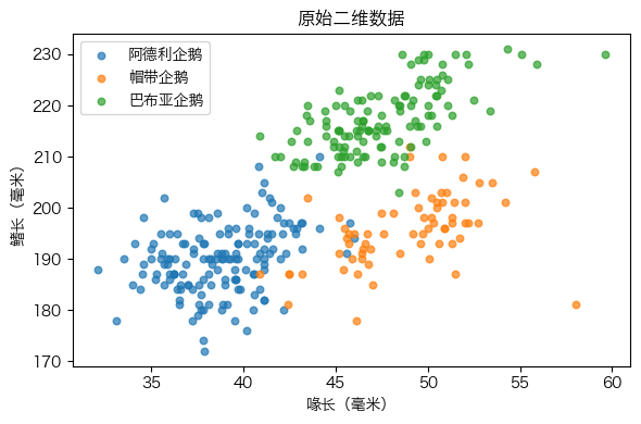
喙长单位是毫米,鳍长也为毫米但范围不同;散点图可见物种簇有重叠和不同位置。生成模型学习的是训练样本的联合分布,不等于物种的“真实自然分布”,因为采样地点、年份与缺失机制都会影响数据。
类别数量不完全相等。后续条件采样给每类相同的生成数量,是为了可视化模型行为,不是估计自然界物种比例。
summary = frame.groupby("species")[features].agg(["count", "mean", "std"])
summary = summary.rename(index={name: class_display[name] for name in class_names})
feature_display = {"bill_length_mm": "喙长(毫米)", "flipper_length_mm": "鳍长(毫米)"}
stat_display = {"count": "样本数", "mean": "均值", "std": "标准差"}
summary.columns = pd.MultiIndex.from_tuples(
    [(feature_display[feature], stat_display[stat]) for feature, stat in summary.columns]
)
display(summary)
fig, ax = plt.subplots(figsize=(6, 4))
for species, group in frame.groupby("species"):
    ax.scatter(group[features[0]], group[features[1]], s=22, alpha=0.7, label=class_display[species])
ax.set(xlabel="喙长(毫米)", ylabel="鳍长(毫米)", title="原始二维数据")
ax.legend()
plt.tight_layout()
| 喙长(毫米) | 鳍长(毫米) | |||||
|---|---|---|---|---|---|---|
| 样本数 | 均值 | 标准差 | 样本数 | 均值 | 标准差 | |
| species | ||||||
| 阿德利企鹅 | 151 | 38.791391 | 2.663405 | 151 | 189.953642 | 6.539457 |
| 帽带企鹅 | 68 | 48.833824 | 3.339256 | 68 | 195.823529 | 7.131894 |
| 巴布亚企鹅 | 123 | 47.504878 | 3.081857 | 123 | 217.186992 | 6.484976 |
第 3 步:无泄漏划分与训练集标准化#
先按类别比例划分训练集、验证集和测试集,再用训练集估计标准化所需的均值与标准差。若先在全部数据上计算这些量,就会把测试集的分布信息提前带入数据处理过程。
条件标签 \(c\in\{0,1,2\}\) 与连续向量 \(\boldsymbol{x}_0\in\mathbb{R}^2\) 分开保存。快速模式使用较小的批次和较少的训练轮次;由于数据只有约 300 行,完整模式主要增加参数更新次数,不会增加额外数据。
X_raw = frame[features].to_numpy(np.float32)
y_raw = frame["class_id"].to_numpy(np.int64)
X_train_raw, X_temp_raw, y_train, y_temp = train_test_split(
    X_raw, y_raw, test_size=0.40, stratify=y_raw, random_state=SEED
)
X_valid_raw, X_test_raw, y_valid, y_test = train_test_split(
    X_temp_raw, y_temp, test_size=0.50, stratify=y_temp, random_state=SEED
)
scaler = StandardScaler().fit(X_train_raw)
X_train = scaler.transform(X_train_raw).astype(np.float32)
X_valid = scaler.transform(X_valid_raw).astype(np.float32)
X_test = scaler.transform(X_test_raw).astype(np.float32)

train_dataset = TensorDataset(torch.from_numpy(X_train), torch.from_numpy(y_train))
generator = torch.Generator().manual_seed(SEED)
train_loader = DataLoader(train_dataset, batch_size=64, shuffle=True, generator=generator)
valid_tensor = (torch.from_numpy(X_valid).to(device), torch.from_numpy(y_valid).to(device))
test_tensor = (torch.from_numpy(X_test).to(device), torch.from_numpy(y_test).to(device))
print({"训练集": X_train.shape, "验证集": X_valid.shape, "测试集": X_test.shape,
       "训练均值": X_train.mean(0), "训练标准差": X_train.std(0)})
{'训练集': (205, 2), '验证集': (68, 2), '测试集': (69, 2), '训练均值': array([ 2.9068167e-07, -1.3258399e-07], dtype=float32), '训练标准差': array([0.9999998, 1.0000001], dtype=float32)}
第 4 步:可解释的高斯条件基线与解析分数#
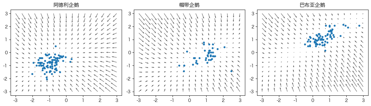
先为每个物种在训练集拟合一个二维高斯。它既是生成基线,也是分数函数的“已知答案”。对高斯
这个向量把远离均值的点拉向高密度椭圆中心。真实类别可能非高斯,所以神经分数模型相对它的价值在于表达弯曲、多峰分布;但在小数据上,更复杂不一定更可靠。
gaussian_parameters = {}
for class_id, name in enumerate(class_names):
    values = X_train[y_train == class_id]
    mean = values.mean(axis=0)
    covariance = np.cov(values.T) + 1e-3 * np.eye(2)
    gaussian_parameters[class_id] = (mean, covariance)

def gaussian_score(points, class_id):
    mean, covariance = gaussian_parameters[class_id]
    return -(points - mean) @ np.linalg.inv(covariance).T

grid_x, grid_y = np.meshgrid(np.linspace(-3, 3, 17), np.linspace(-3, 3, 17))
grid = np.c_[grid_x.ravel(), grid_y.ravel()]
fig, axes = plt.subplots(1, 3, figsize=(12, 3.5))
for class_id, axis in enumerate(axes):
    vector = gaussian_score(grid, class_id)
    axis.quiver(grid[:, 0], grid[:, 1], vector[:, 0], vector[:, 1], alpha=0.65)
    axis.scatter(X_train[y_train == class_id, 0], X_train[y_train == class_id, 1], s=12)
    axis.set_title(class_display[class_names[class_id]])
plt.tight_layout()
第 5 步:方差保持与方差爆炸随机微分方程,以及反向时间#
连续扩散写成
方差保持 SDE:\(\boldsymbol{f}=-\frac{1}{2}\beta(t)\boldsymbol{x}\),\(g=\sqrt{\beta(t)}\),总方差受控,与 DDPM 的连续时间极限紧密相关;
方差爆炸 SDE:\(\boldsymbol{f}=\boldsymbol{0}\),噪声尺度持续增大,数据方差不会被信号缩放抵消。
已知时间边缘分数 \(\boldsymbol{s}_t(\boldsymbol{x})=\nabla_{\boldsymbol{x}}\log p_t(\boldsymbol{x})\) 后,反向时间 SDE 的漂移变为 \(\boldsymbol{f}-g^2\boldsymbol{s}_t\),仍然含有随机项;概率流 ODE 使用 \(\boldsymbol{f}-\frac{1}{2}g^2\boldsymbol{s}_t\),不含随机项,并且与 SDE 具有相同的时间边缘分布。理解符号方向时,必须同时注意“积分从较大的 \(t\) 走向较小的 \(t\)”,不能只背公式。
def beta_continuous(t, beta_min=0.1, beta_max=20.0):
    return beta_min + t * (beta_max - beta_min)

def vp_drift_diffusion(x, t):
    beta_t = beta_continuous(t)
    drift = -0.5 * beta_t[:, None] * x
    diffusion = torch.sqrt(beta_t)
    return drift, diffusion

def ve_sigma(t, sigma_min=0.01, sigma_max=20.0):
    return sigma_min * (sigma_max / sigma_min) ** t

probe_x = torch.tensor([[1.0, -1.0], [0.5, 0.2]])
probe_t = torch.tensor([0.1, 0.9])
drift, diffusion = vp_drift_diffusion(probe_x, probe_t)
print("方差保持过程中漂移项与扩散系数的维度:", drift.shape, diffusion.shape)
print("方差爆炸过程噪声尺度:", ve_sigma(probe_t))
方差保持过程中漂移项与扩散系数的维度: torch.Size([2, 2]) torch.Size([2])
方差爆炸过程噪声尺度: tensor([0.0214, 9.3525])
第 6 步:离散 VP 过程与分数—噪声等价#
为了随后使用 DDPM/DDIM,我们采用离散的 VP 加噪参数设置:
条件于干净样本的扰动核分数为
因此,预测噪声 \(\boldsymbol{\epsilon}_\theta\) 等价于预测分数 \(\boldsymbol{s}_\theta=-\boldsymbol{\epsilon}_\theta/\sigma_t\)。去噪分数匹配通常乘以 \(\sigma_t^2\) 来平衡不同噪声尺度下的数值大小,恰好得到噪声的均方误差(mean squared error,MSE)。
T = 60 if FAST_MODE else 200
betas = torch.linspace(1e-4, 0.08 if FAST_MODE else 0.02, T, device=device)
alphas = 1.0 - betas
alpha_bar = torch.cumprod(alphas, dim=0)

def extract(vector, t, x):
    return vector.gather(0, t).reshape(-1, 1).to(x.dtype)

def q_sample(x0, t, noise=None):
    noise = torch.randn_like(x0) if noise is None else noise
    mean = extract(alpha_bar.sqrt(), t, x0) * x0
    sigma = extract((1 - alpha_bar).sqrt(), t, x0)
    return mean + sigma * noise, noise

x0_probe = torch.from_numpy(X_train[:8]).to(device)
t_probe = torch.arange(8, device=device) * (T // 8)
noise_probe = torch.randn_like(x0_probe)
xt_probe, epsilon_probe = q_sample(x0_probe, t_probe, noise_probe)
sigma_probe = extract((1 - alpha_bar).sqrt(), t_probe, x0_probe)
conditional_score = -(xt_probe - extract(alpha_bar.sqrt(), t_probe, x0_probe) * x0_probe) / sigma_probe.pow(2)
assert torch.allclose(conditional_score, -epsilon_probe / sigma_probe, atol=1e-5)
print("分数—噪声比例的数值检查通过,维度:", conditional_score.shape)
分数—噪声比例的数值检查通过,维度: torch.Size([8, 2])
第 7 步:类别条件与无分类器引导#
条件模型接收 \((\boldsymbol{x}_t,t,c)\)。训练时以概率 \(p_{\mathrm{drop}}\) 把类别替换为“空条件”,因此同一个网络同时学习:
\(\boldsymbol{\epsilon}_\theta(\boldsymbol{x}_t,t,c)\):条件预测;
\(\boldsymbol{\epsilon}_\theta(\boldsymbol{x}_t,t,\varnothing)\):无条件预测。
采样时 CFG 组合
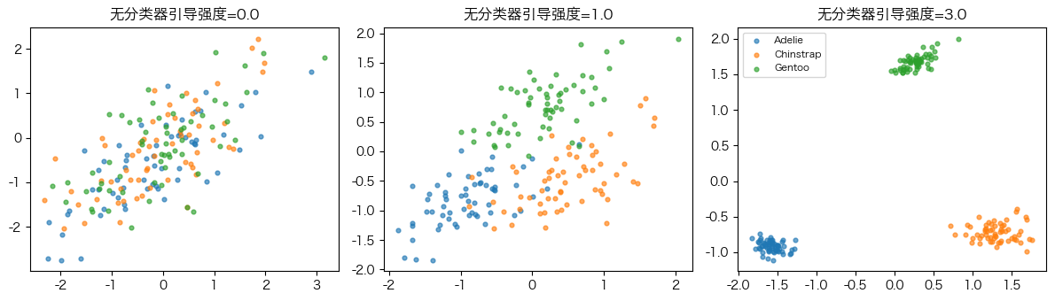
\(w=0\) 对应无条件预测,\(w=1\) 对应普通条件预测;更大的 \(w\) 会放大条件与无条件预测之差,但可能降低多样性,并把样本推离真实数据的高密度区域。空条件是额外的嵌入编号,不代表某个真实物种。
class TimeEmbedding(torch.nn.Module):
    def __init__(self, dimension):
        super().__init__()
        self.dimension = dimension

    def forward(self, t):
        half = self.dimension // 2
        frequency = torch.exp(
            -np.log(10000) * torch.arange(half, device=t.device) / max(half - 1, 1)
        )
        angles = t.float()[:, None] * frequency[None]
        return torch.cat([angles.sin(), angles.cos()], dim=1)

class ConditionalNoiseMLP(torch.nn.Module):
    def __init__(self, classes=3, hidden=96):
        super().__init__()
        self.null_class = classes
        self.time_embedding = TimeEmbedding(32)
        self.class_embedding = torch.nn.Embedding(classes + 1, 16)
        self.net = torch.nn.Sequential(
            torch.nn.Linear(2 + 32 + 16, hidden),
            torch.nn.SiLU(),
            torch.nn.Linear(hidden, hidden),
            torch.nn.SiLU(),
            torch.nn.Linear(hidden, 2),
        )

    def forward(self, x, t, condition):
        combined = torch.cat([x, self.time_embedding(t), self.class_embedding(condition)], dim=1)
        return self.net(combined)

model = ConditionalNoiseMLP(len(class_names), 80 if FAST_MODE else 128).to(device)
shape_output = model(
    torch.zeros(5, 2, device=device),
    torch.arange(5, device=device),
    torch.tensor([0, 1, 2, 3, 3], device=device),
)
assert shape_output.shape == (5, 2)
print("条件模型输出的维度核验:", shape_output.shape, "空条件编号:", model.null_class)
条件模型输出的维度核验: torch.Size([5, 2]) 空条件编号: 3
第 8 步:去噪分数匹配训练#
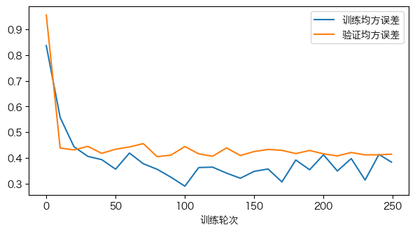
每个批次随机选择 t 和噪声,10% 条件被替换为空条件。损失只用训练集;验证集使用固定随机数流,保存最低验证噪声均方误差(MSE)的状态。
快速模式约 250 个训练轮次,但每轮只有几个极小批次;完整模式提高隐藏宽度与训练次数。二维小样本的训练波动明显,严肃比较仍应运行多个种子。
optimizer = torch.optim.AdamW(model.parameters(), lr=2e-3)
epochs = 250 if FAST_MODE else 800
drop_probability = 0.10

def training_loss(x0, condition):
    t = torch.randint(0, T, (len(x0),), device=device)
    xt, noise = q_sample(x0, t)
    dropped = condition.clone()
    mask = torch.rand(len(condition), device=device) < drop_probability
    dropped[mask] = model.null_class
    return torch.nn.functional.mse_loss(model(xt, t, dropped), noise)

@torch.no_grad()
def validation_loss():
    model.eval()
    x0, condition = valid_tensor
    generator = torch.Generator(device=device).manual_seed(SEED + 10)
    t = torch.randint(0, T, (len(x0),), generator=generator, device=device)
    noise = torch.randn(x0.shape, generator=generator, device=device)
    xt, _ = q_sample(x0, t, noise)
    return float(torch.nn.functional.mse_loss(model(xt, t, condition), noise))

records, best_state, best_valid = [], None, float("inf")
for epoch in range(epochs):
    model.train()
    losses = []
    for x0, condition in train_loader:
        x0, condition = x0.to(device), condition.to(device)
        optimizer.zero_grad()
        loss = training_loss(x0, condition)
        loss.backward()
        torch.nn.utils.clip_grad_norm_(model.parameters(), 2.0)
        optimizer.step()
        losses.append(loss.item())
    if epoch % 10 == 0 or epoch == epochs - 1:
        valid = validation_loss()
        records.append({"训练轮次": epoch, "训练均方误差": np.mean(losses), "验证均方误差": valid})
        if valid < best_valid:
            best_valid = valid
            best_state = copy.deepcopy(model.state_dict())
model.load_state_dict(best_state)
history = pd.DataFrame(records)
display(history.tail())
history.plot(x="训练轮次", y=["训练均方误差", "验证均方误差"], figsize=(7, 3.5));
| 训练轮次 | 训练均方误差 | 验证均方误差 | |
|---|---|---|---|
| 21 | 210 | 0.349276 | 0.407845 |
| 22 | 220 | 0.397449 | 0.421135 |
| 23 | 230 | 0.314072 | 0.412062 |
| 24 | 240 | 0.413636 | 0.412066 |
| 25 | 249 | 0.383754 | 0.414770 |
第 9 步:确定模型与训练方案后评价分数方向#
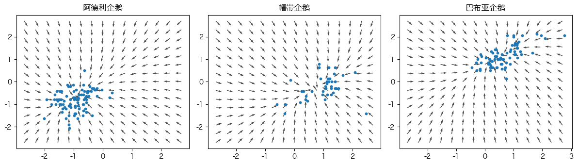
测试噪声 MSE 检查噪声预测这一间接任务;更切合本案例的检查是:在噪声较小的时间步,学习到的分数是否大致指向相应类别的高密度区域。我们把网络预测的噪声转换成 \(\boldsymbol{s}_\theta=-\boldsymbol{\epsilon}_\theta/\sigma_t\),再画出向量场。
向量场只在训练数据覆盖区域附近可信;远离数据的外推箭头可能任意。若箭头整体过大或方向杂乱,通常意味着训练不足、t 太靠近 0 导致除以很小的 sigma,或模型容量不合适。
@torch.no_grad()
def fixed_noise_mse(x0, condition):
    generator = torch.Generator(device=device).manual_seed(SEED + 20)
    t = torch.randint(0, T, (len(x0),), generator=generator, device=device)
    noise = torch.randn(x0.shape, generator=generator, device=device)
    xt, _ = q_sample(x0, t, noise)
    return float(torch.nn.functional.mse_loss(model(xt, t, condition), noise))

test_mse = fixed_noise_mse(*test_tensor)
print("最终测试噪声均方误差:", test_mse)

@torch.no_grad()
def learned_score(points, class_id, time_index=2):
    x = torch.as_tensor(points, dtype=torch.float32, device=device)
    t = torch.full((len(x),), time_index, dtype=torch.long, device=device)
    condition = torch.full((len(x),), class_id, dtype=torch.long, device=device)
    epsilon = model(x, t, condition)
    sigma = extract((1 - alpha_bar).sqrt(), t, x)
    return (-epsilon / sigma).cpu().numpy()

field_grid_x, field_grid_y = np.meshgrid(np.linspace(-2.7, 2.7, 15), np.linspace(-2.7, 2.7, 15))
field_grid = np.c_[field_grid_x.ravel(), field_grid_y.ravel()]
fig, axes = plt.subplots(1, 3, figsize=(12, 3.5))
for class_id, axis in enumerate(axes):
    vector = learned_score(field_grid, class_id, time_index=max(2, T // 20))
    norm = np.linalg.norm(vector, axis=1, keepdims=True)
    vector = vector / np.maximum(norm, 1.0)
    axis.quiver(field_grid[:, 0], field_grid[:, 1], vector[:, 0], vector[:, 1], alpha=0.7)
    axis.scatter(X_train[y_train == class_id, 0], X_train[y_train == class_id, 1], s=10)
    axis.set_title(class_display[class_names[class_id]])
plt.tight_layout()
最终测试噪声均方误差: 0.4368978440761566
第 10 步:去噪扩散隐式模型把随机反向链改成可控的非马尔可夫路径#
先由噪声预测恢复
从 t 跳到更早的 s 时,DDIM 更新为
\(\eta=0\) 时 \(\sigma=0\),给定初始噪声后路径确定,可跳过大量时间步;\(\eta>0\) 恢复随机性。DDIM 加速的是采样,不意味着训练也能少看噪声等级。
@torch.no_grad()
def guided_noise(x, t, condition, guidance):
    null = torch.full_like(condition, model.null_class)
    epsilon_unconditional = model(x, t, null)
    epsilon_conditional = model(x, t, condition)
    return epsilon_unconditional + guidance * (epsilon_conditional - epsilon_unconditional)

@torch.no_grad()
def ddim_step(x, t_index, previous_index, condition, guidance=1.0, eta=0.0):
    t = torch.full((len(x),), t_index, dtype=torch.long, device=device)
    epsilon = guided_noise(x, t, condition, guidance)
    current_bar = alpha_bar[t_index]
    previous_bar = torch.tensor(1.0, device=device) if previous_index < 0 else alpha_bar[previous_index]
    x0_hat = (x - torch.sqrt(1 - current_bar) * epsilon) / torch.sqrt(current_bar)
    sigma = eta * torch.sqrt(
        ((1 - previous_bar) / (1 - current_bar) * (1 - current_bar / previous_bar)).clamp_min(0)
    )
    direction = torch.sqrt((1 - previous_bar - sigma ** 2).clamp_min(0)) * epsilon
    return torch.sqrt(previous_bar) * x0_hat + direction + sigma * torch.randn_like(x)

@torch.no_grad()
def sample_ddim(per_class=80, guidance=1.0, steps=15, eta=0.0, initial=None):
    condition = torch.arange(len(class_names), device=device).repeat_interleave(per_class)
    x = torch.randn(len(condition), 2, device=device) if initial is None else initial.clone().to(device)
    sequence = np.unique(np.linspace(0, T - 1, steps, dtype=int))[::-1]
    for position, time_index in enumerate(sequence):
        previous = int(sequence[position + 1]) if position + 1 < len(sequence) else -1
        x = ddim_step(x, int(time_index), previous, condition, guidance, eta)
    return x.cpu().numpy(), condition.cpu().numpy()
第 11 步:比较 CFG 强度与 DDIM 采样步数#
在其他条件相同的情况下,先使用完全相同的初始噪声,只改变引导强度,以便分析条件强度可能带来的影响。我们比较 0、1 和 3:
0:空条件生成;
1:普通条件预测;
3:放大条件方向。
随后固定引导强度,比较 8 与 30 个 DDIM 步。更少步更快,但数值离散误差可能更大;小数据模型本身的误差也可能主导结果。评价先用可视化和“离对应训练类中心的距离”,后者只是粗略教学指标,不是分布质量的完整度量。
per_class = 60
initial_generator = torch.Generator(device=device).manual_seed(SEED + 30)
initial = torch.randn(len(class_names) * per_class, 2, generator=initial_generator, device=device)

fig, axes = plt.subplots(1, 3, figsize=(12, 3.5))
guidance_rows = []
for guidance, axis in zip([0.0, 1.0, 3.0], axes):
    samples, labels = sample_ddim(per_class, guidance=guidance, steps=15, eta=0.0, initial=initial)
    for class_id, name in enumerate(class_names):
        subset = samples[labels == class_id]
        axis.scatter(subset[:, 0], subset[:, 1], s=12, alpha=0.65, label=name)
        center = X_train[y_train == class_id].mean(0)
        guidance_rows.append({
            "引导强度": guidance,
            "类别": class_display[name],
            "到训练类中心的平均距离": float(np.linalg.norm(subset - center, axis=1).mean()),
        })
    axis.set_title(f"无分类器引导强度={guidance}")
axes[-1].legend(fontsize=8)
plt.tight_layout()
display(pd.DataFrame(guidance_rows))

for step_count in [8, 30]:
    samples, labels = sample_ddim(per_class, guidance=1.0, steps=step_count, eta=0.0, initial=initial)
    print("去噪扩散隐式模型采样步数", step_count, "样本均值", samples.mean(0), "样本标准差", samples.std(0))
| 引导强度 | 类别 | 到训练类中心的平均距离 | |
|---|---|---|---|
| 0 | 0.0 | 阿德利企鹅 | 1.362322 |
| 1 | 0.0 | 帽带企鹅 | 1.522064 |
| 2 | 0.0 | 巴布亚企鹅 | 1.837931 |
| 3 | 1.0 | 阿德利企鹅 | 0.568229 |
| 4 | 1.0 | 帽带企鹅 | 0.790616 |
| 5 | 1.0 | 巴布亚企鹅 | 0.812164 |
| 6 | 3.0 | 阿德利企鹅 | 0.649138 |
| 7 | 3.0 | 帽带企鹅 | 0.617272 |
| 8 | 3.0 | 巴布亚企鹅 | 0.658310 |
去噪扩散隐式模型采样步数 8 样本均值 [-0.07687686 -0.18400334] 样本标准差 [0.8091002  0.81972903]
去噪扩散隐式模型采样步数 30 样本均值 [-0.07143474 -0.16645573] 样本标准差 [0.8322108  0.83575106]
第 12 步:朗之万动力学、反向随机微分方程与概率流常微分方程的联系#
若直接获得某噪声尺度的分数,朗之万(Langevin)更新为
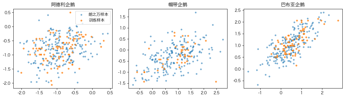
随机项帮助探索分布;删去随机项只做梯度上升,容易收缩到众数。反向 SDE 同样含随机扩散项,而概率流 ODE 是确定性路径。DDIM 的 \(\eta=0\) 与“确定性概率流”在直觉上相近,但离散参数化和推导路径不同,不能简单说两者处处完全相同。
下面用解析高斯分数做短 Langevin 演示,排除神经网络误差,观察随机粒子向类别分布移动。
def langevin_gaussian(class_id, particles=200, steps=80, step_size=0.025):
    generator = torch.Generator().manual_seed(SEED + class_id)
    x = torch.randn(particles, 2, generator=generator) * 3
    mean, covariance = gaussian_parameters[class_id]
    precision = torch.from_numpy(np.linalg.inv(covariance)).float()
    center = torch.from_numpy(mean).float()
    for _ in range(steps):
        score = -(x - center) @ precision.T
        x = x + 0.5 * step_size * score + np.sqrt(step_size) * torch.randn(
            x.shape, generator=generator
        )
    return x.numpy()

fig, axes = plt.subplots(1, 3, figsize=(12, 3.5))
for class_id, axis in enumerate(axes):
    particles = langevin_gaussian(class_id)
    axis.scatter(particles[:, 0], particles[:, 1], s=10, alpha=0.5, label="朗之万样本")
    axis.scatter(X_train[y_train == class_id, 0], X_train[y_train == class_id, 1],
                 s=12, alpha=0.7, label="训练样本")
    axis.set_title(class_display[class_names[class_id]])
axes[0].legend()
plt.tight_layout()
第 13 步:迁移到 Fashion-MNIST 时,哪些部分改变#
二维 MLP 会换成图像网络,但训练随机变量和公式不变:
\(\boldsymbol{x}\):从 \((B,2)\) 变为 \((B,1,28,28)\);
时间系数:从 \((B,1)\) 重塑为 \((B,1,1,1)\);
类别嵌入:仍可通过加法、特征线性调制(feature-wise linear modulation,FiLM)或交叉注意力进入网络;
U-Net 使用多尺度卷积与跳连;LDM 先由变分自编码器(variational autoencoder,VAE)把图像压缩成潜变量,再在潜空间执行扩散;DiT 用 Transformer 处理潜变量图像块。
下面只通过不需登录的公开链接下载 Fashion-MNIST 的训练图像与标签,解析 64 张图像进行维度检查,不训练图像模型。这样可以区分“核心算法已经运行”和“高维扩展仍需大量计算资源”。
FASHION_URLS = {
    "images": "https://storage.googleapis.com/tensorflow/tf-keras-datasets/train-images-idx3-ubyte.gz",
    "labels": "https://storage.googleapis.com/tensorflow/tf-keras-datasets/train-labels-idx1-ubyte.gz",
}
fashion_paths = {
    name: download_cached(url, cache_root / Path(url).name)
    for name, url in FASHION_URLS.items()
}

with gzip.open(fashion_paths["images"], "rb") as handle:
    magic, count, rows, cols = struct.unpack(">IIII", handle.read(16))
    image_bytes = np.frombuffer(handle.read(64 * rows * cols), dtype=np.uint8).copy()
with gzip.open(fashion_paths["labels"], "rb") as handle:
    label_magic, label_count = struct.unpack(">II", handle.read(8))
    label_bytes = np.frombuffer(handle.read(64), dtype=np.uint8).copy()

fashion_x = torch.from_numpy(image_bytes.reshape(64, 1, rows, cols)).float() / 127.5 - 1
fashion_y = torch.from_numpy(label_bytes.astype(np.int64))
assert magic == 2051 and label_magic == 2049
assert fashion_x.shape == (64, 1, 28, 28)
print("图像扩展输入:", fashion_x.shape, "条件:", fashion_y.shape)
image_t = torch.arange(64, device=alpha_bar.device) % len(alpha_bar)
coefficient_shape = alpha_bar[image_t].reshape(64, 1, 1, 1).shape
print("图像广播所需时间系数的维度:", coefficient_shape)
文件: train-images-idx3-ubyte.gz ;SHA-256: 3aede38d61863908ad78613f6a32ed271626dd12800ba2636569512369268a84
文件: train-labels-idx1-ubyte.gz ;SHA-256: a04f17134ac03560a47e3764e11b92fc97de4d1bfaf8ba1a3aa29af54cc90845
图像扩展输入: torch.Size([64, 1, 28, 28]) 条件: torch.Size([64])
图像广播所需时间系数的维度: torch.Size([64, 1, 1, 1])
结论、局限与常见错误#
本案例用二维真实数据把分数场、条件引导和确定/随机采样路径可视化,并明确高维网络只是表示层面的扩展。局限包括:
企鹅数据很小,二维条件分布估计不稳定,不能作生态结论;
类中心距离会奖励收缩,无法衡量覆盖度和多样性;
CFG 的高权重可能让类更分离,同时牺牲真实度;必须多指标评价;
DDIM 的少步实验混合模型误差与数值离散误差;
图像部分只核对数据与各个量的维度,没有训练 U-Net、LDM 或 DiT;
分类器引导未单独实现:它需要额外的带噪分类器梯度;本案例实现的是 CFG,二者不能混称。
常见错误:把分数函数当类别概率、漏掉 \(-1/\sigma_t\) 比例、反向积分时弄错时间方向、把 CFG 的 \(w=0\) 误写为普通条件、用不同初始噪声比较引导强度、声称 DDIM 不需训练扩散模型,以及把潜空间压缩造成的误差归于扩散过程本身。
综合练习#
对解析高斯分数做有限差分:比较 \(\nabla_x\log p(x)\) 与 gaussian_score。
固定初始粒子,比较随机 Langevin、反向 SDE 和确定概率流 ODE 的轨迹方差。
对 CFG \(w\in\{0,0.5,1,2,4\}\) 运行多个初始噪声,同时评价中心距离、协方差误差和最近邻距离。
实现一个独立带噪分类器,并用 \(\nabla_x\log p(c\mid x_t)\) 完成分类器引导;与 CFG 比较额外训练成本。
将同一核心代码迁移到 Fashion-MNIST 小型 U-Net,逐层核对各个量的维度;再解释 VAE 潜变量和 DiT 图像块分别改变了什么、没有改变什么。